Make Joins on Geographical Data: Spatial Support in Databricks
Databricks Runtime 17.1 introduces powerful geospatial support, featuring new Delta datatypes: geography and geometry, along with dozens of ST spatial functions. This makes it incredibly easy to perform joins on geographical data, such as connecting delivery locations with their corresponding delivery zones or cities.
Understanding Coordinate Reference Systems
You'll frequently encounter two standard codes in datatypes and error messages: 4326 and CRS84. Both describe the WGS 84 coordinate reference system, which uses latitude and longitude to locate positions on Earth.
EPSG:4326 is the official SRID (Spatial Reference System Identifier), while CRS84 is an equivalent definition used by OGC/WKT, with longitude–latitude axis order. The GEOGRAPHY type in Databricks always uses SRID 4326. The GEOMETRY type can use various SRIDs, or even none at all, since it can represent abstract x–y coordinate systems that aren't tied to the Earth.
Setting Up Delivery Zones
Let's start by creating a map with our cities (delivery zones):
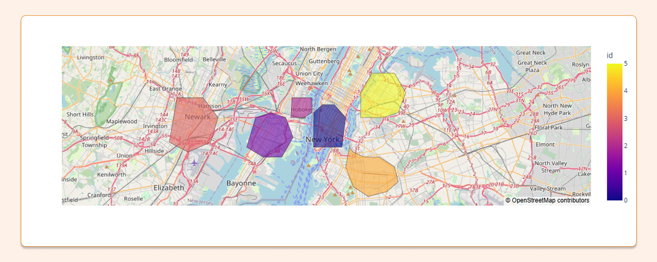
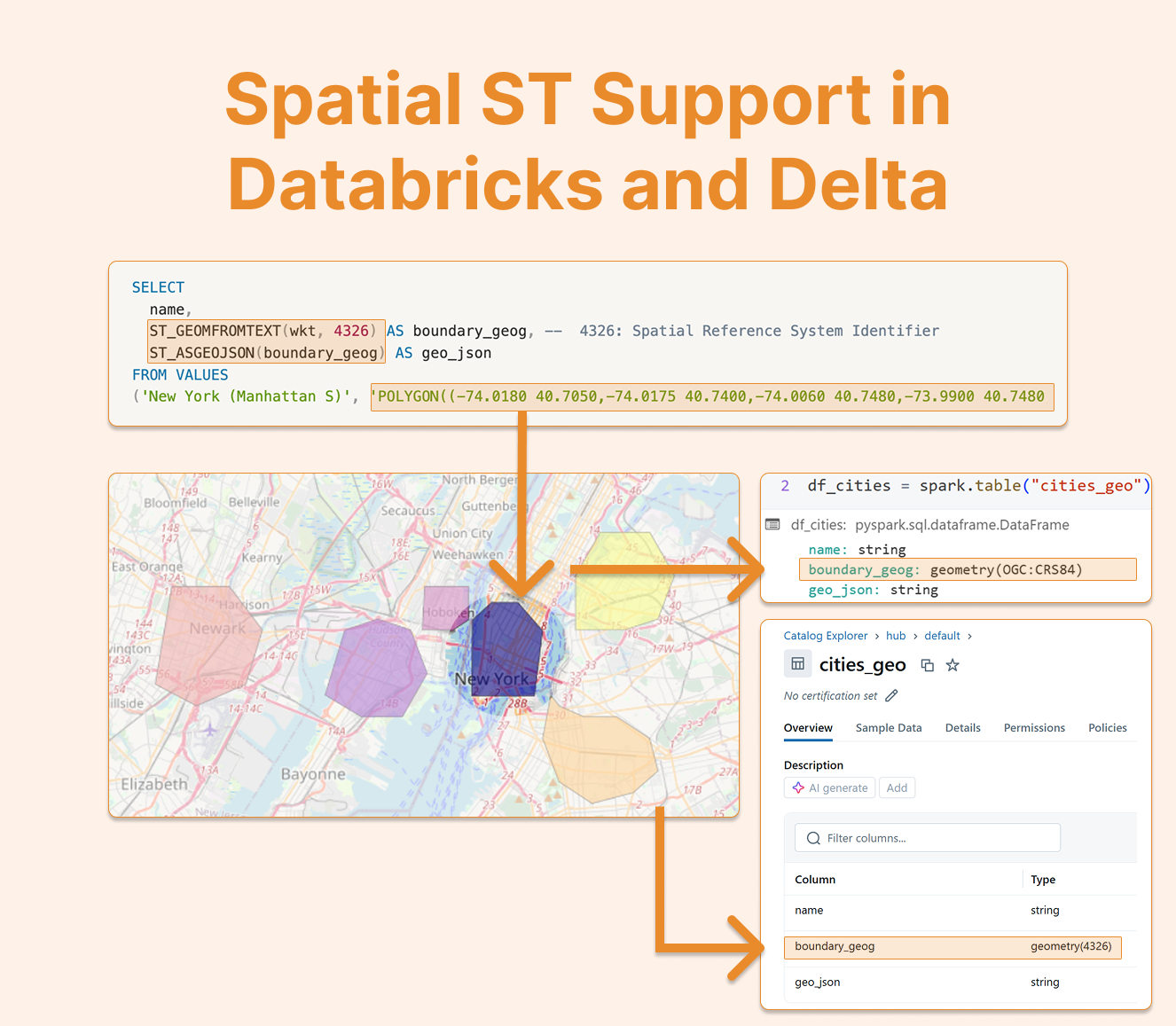
This represents exactly what we define in our temporary view: polygons with latitude/longitude points stored in the GEOGRAPHY type. We can also store this data as a JSON string for other uses.
CREATE OR REPLACE TEMP VIEW cities_geo AS
SELECT
name,
ST_GEOMFROMTEXT(wkt, 4326) AS boundary_geog, -- 4326: Spatial Reference System Identifier
ST_ASGEOJSON(boundary_geog) AS geo_json
FROM VALUES
('New York (Manhattan S)', 'POLYGON((-74.0180 40.7050,-74.0175 40.7400,-74.0060 40.7480,-73.9900 40.7480,-73.9750 40.7350,-73.9800 40.7050,-74.0180 40.7050))'),
('Jersey City', 'POLYGON((-74.1070 40.7050,-74.0950 40.7350,-74.0750 40.7400,-74.0550 40.7350,-74.0450 40.7150,-74.0600 40.6950,-74.0850 40.6950,-74.1070 40.7050))'),
('Hoboken', 'POLYGON((-74.0480 40.7350,-74.0465 40.7550,-74.0200 40.7550,-74.0200 40.7400,-74.0300 40.7350,-74.0480 40.7350))'),
('Newark', 'POLYGON((-74.2100 40.7100,-74.2000 40.7550,-74.1650 40.7550,-74.1450 40.7350,-74.1550 40.7100,-74.1850 40.7000,-74.2100 40.7100))'),
('Brooklyn (Central)', 'POLYGON((-73.9700 40.7050,-73.9650 40.7000,-73.9500 40.6950,-73.9300 40.6950,-73.9100 40.6850,-73.9050 40.6700,-73.9200 40.6600,-73.9450 40.6550,-73.9650 40.6650,-73.9750 40.6850,-73.9700 40.7050))'),
('Queens (LIC/Astoria)', 'POLYGON((-73.9550 40.7350,-73.9550 40.7600,-73.9400 40.7800,-73.9100 40.7800,-73.8950 40.7600,-73.9050 40.7400,-73.9250 40.7350,-73.9550 40.7350))')
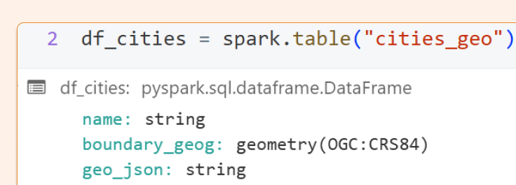
AS t(name, wkt);Notice that our datatype displays as CRS84 in the interface, but after saving in Unity Catalog, it appears as GEOMETRY(4326). Databricks is making an effort to educate users about the relationship between CRS84 and SRID 4326.

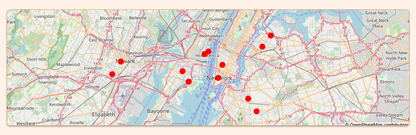
Creating Delivery Points
Now that we have our delivery zones, let's create specific delivery locations. These are simple longitude/latitude points representing food delivery addresses.
CREATE OR REPLACE TEMP VIEW deliveries_geo AS
SELECT
  CAST(id AS INT) AS id,
  CAST(lon AS DOUBLE) AS lon,
  CAST(lat AS DOUBLE) AS lat,
  ST_POINT(lon, lat, 4326) AS pt_geog -- GEOGRAPHY data type
FROM VALUES
  (1, -74.0080, 40.7130),
  (2, -74.0005, 40.7305),
  (3, -74.0710, 40.7220),
  (4, -74.0600, 40.7080),
  (5, -74.0320, 40.7450),
  (6, -74.0250, 40.7485),
  (7, -74.1800, 40.7350),
  (8, -74.1950, 40.7180),
  (9, -73.9550, 40.6850),
  (10, -73.9400, 40.6680),
  (11, -73.9300, 40.7550),
  (12, -73.9150, 40.7700) AS t (id, lon, lat);
Performing Spatial Joins
The beauty of Databricks' geospatial support becomes evident when joining delivery locations with their corresponding cities. This spatial join is surprisingly straightforward:
SELECT
  d.id AS delivery_id,
  c.name AS city_name
FROM deliveries_geo AS d
LEFT JOIN cities_geo AS c
  ON st_contains(c.boundary_geog, d.pt_geog);
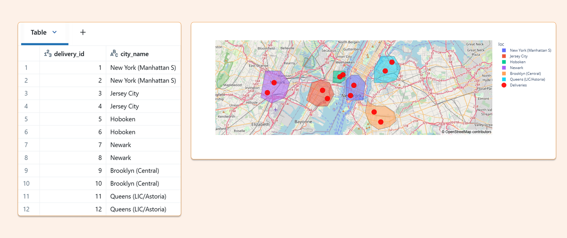
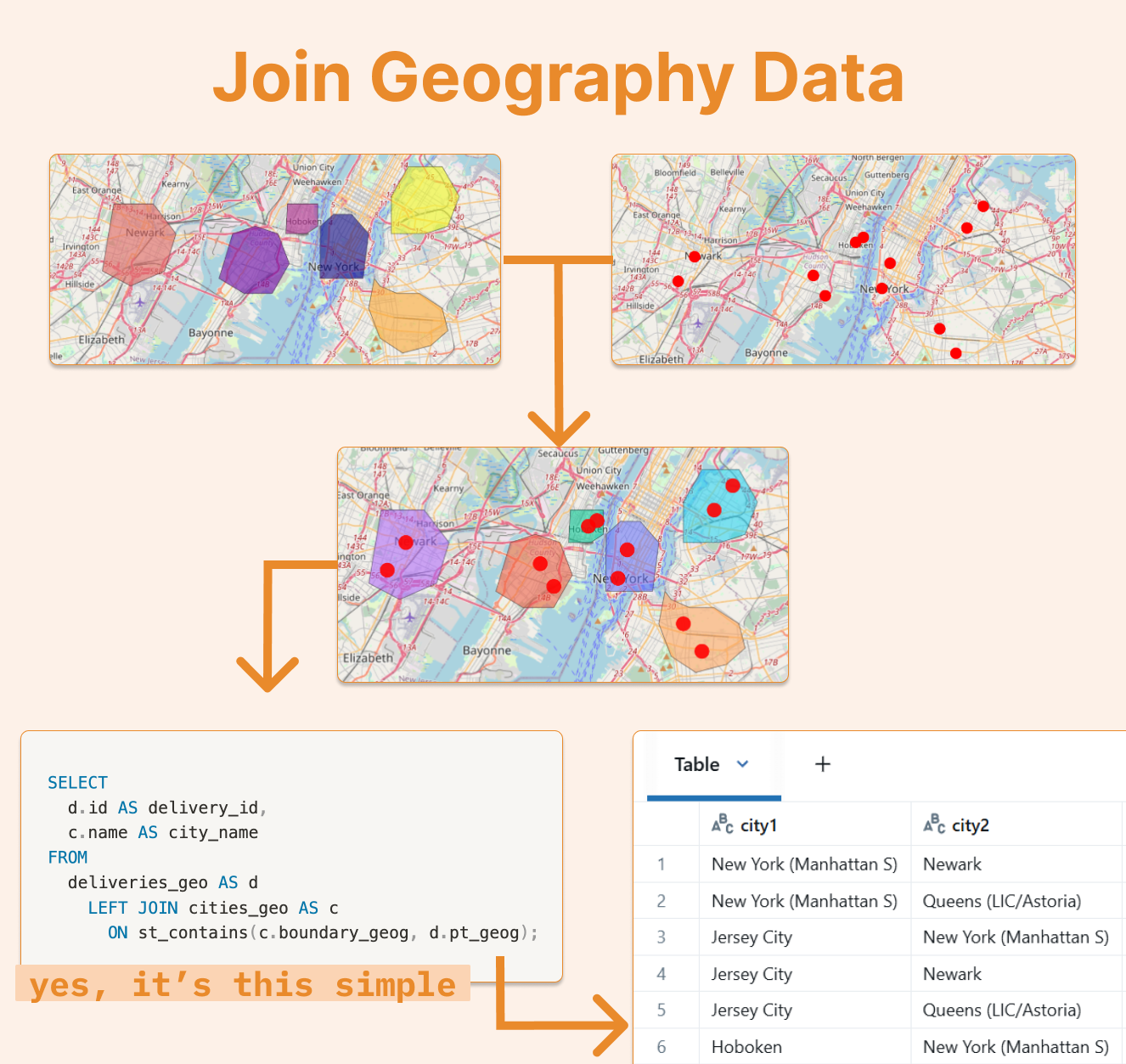
This query uses the ST_CONTAINS function to determine which delivery points fall within each city's boundary polygon.
Going Nerd
Calculating Inter-City Distances
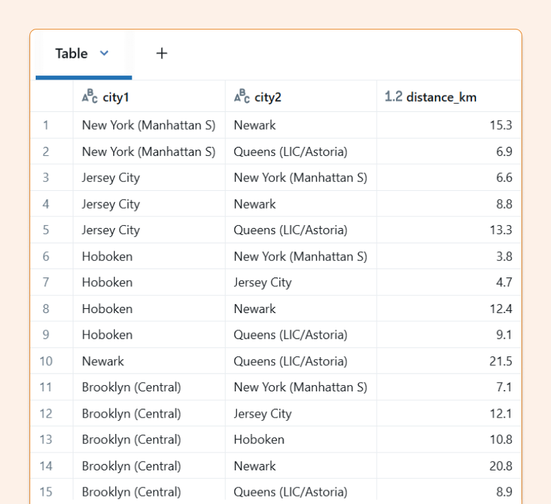
Here's another useful spatial operation: finding the center of each city (polygon) and calculating distances between them:
SELECT
  c1.name AS city1,
  c2.name AS city2,
  ROUND(ST_DISTANCESPHEROID(ST_CENTROID(c1.boundary_geog),
                           ST_CENTROID(c2.boundary_geog)) / 1000, 1) AS distance_km
FROM cities_geo AS c1
CROSS JOIN cities_geo AS c2
WHERE c1.name < c2.name
This query calculates the spheroidal distance between city centers in kilometers.
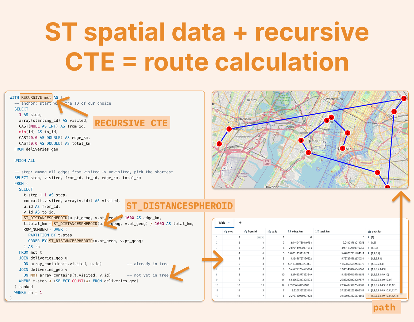
Advanced Example: Minimum Spanning Tree
For those interested in more complex applications, here's a sophisticated example that combines Databricks' new recursive CTE functionality with geospatial functions to implement Prim's algorithm for building a minimum spanning tree of delivery points:
DECLARE OR REPLACE VARIABLE starting_id INT DEFAULT 1;

WITH RECURSIVE mst AS (
  -- Anchor: start with the ID of our choice
  SELECT
    1 AS step,
    array(starting_id) AS visited,
    CAST(NULL AS INT) AS from_id,
    min(id) AS to_id,
    CAST(0.0 AS DOUBLE) AS edge_km,
    CAST(0.0 AS DOUBLE) AS total_km
  FROM deliveries_geo

  UNION ALL

  -- Step: among all edges from visited -> unvisited, pick the shortest
  SELECT step, visited, from_id, to_id, edge_km, total_km
  FROM (
    SELECT
      t.step + 1 AS step,
      concat(t.visited, array(v.id)) AS visited,
      u.id AS from_id,
      v.id AS to_id,
      ST_DISTANCESPHEROID(u.pt_geog, v.pt_geog) / 1000 AS edge_km,
      t.total_km + ST_DISTANCESPHEROID(u.pt_geog, v.pt_geog) / 1000 AS total_km,
      ROW_NUMBER() OVER (
        PARTITION BY t.step
        ORDER BY ST_DISTANCESPHEROID(u.pt_geog, v.pt_geog)
      ) AS rn
    FROM mst t
    JOIN deliveries_geo u
      ON array_contains(t.visited, u.id)           -- already in tree
    JOIN deliveries_geo v
      ON NOT array_contains(t.visited, v.id)       -- not yet in tree
    WHERE t.step < (SELECT COUNT(*) FROM deliveries_geo)
  ) ranked
  WHERE rn = 1
)
SELECT
  step,
  from_id,
  to_id,
  edge_km,
  total_km,
  visited AS path_ids
FROM mst
ORDER BY step;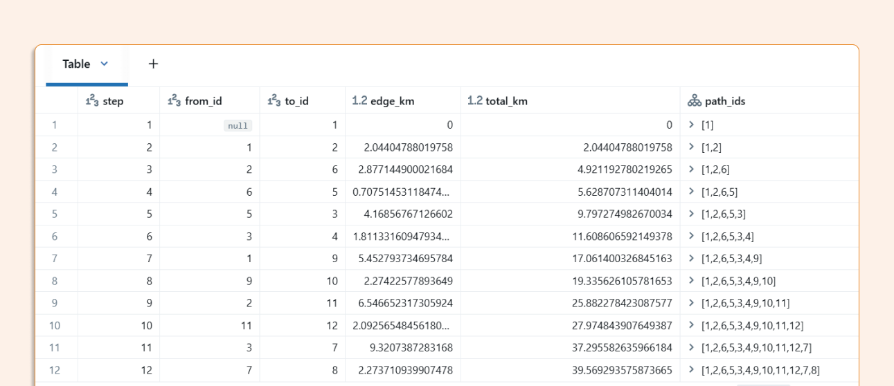
Starting from delivery point 1, this algorithm finds the optimal route: [1, 2, 6, 5, 3, 4, 9, 10, 11, 12, 7, 8]. This represents the most efficient path if you had a helicopter for city-to-city deliveries.
Note: While exploring geographical data in Databricks, you might find it surprisingly easy to exceed the recursive limit of 1 million iterations with complex spatial algorithms.
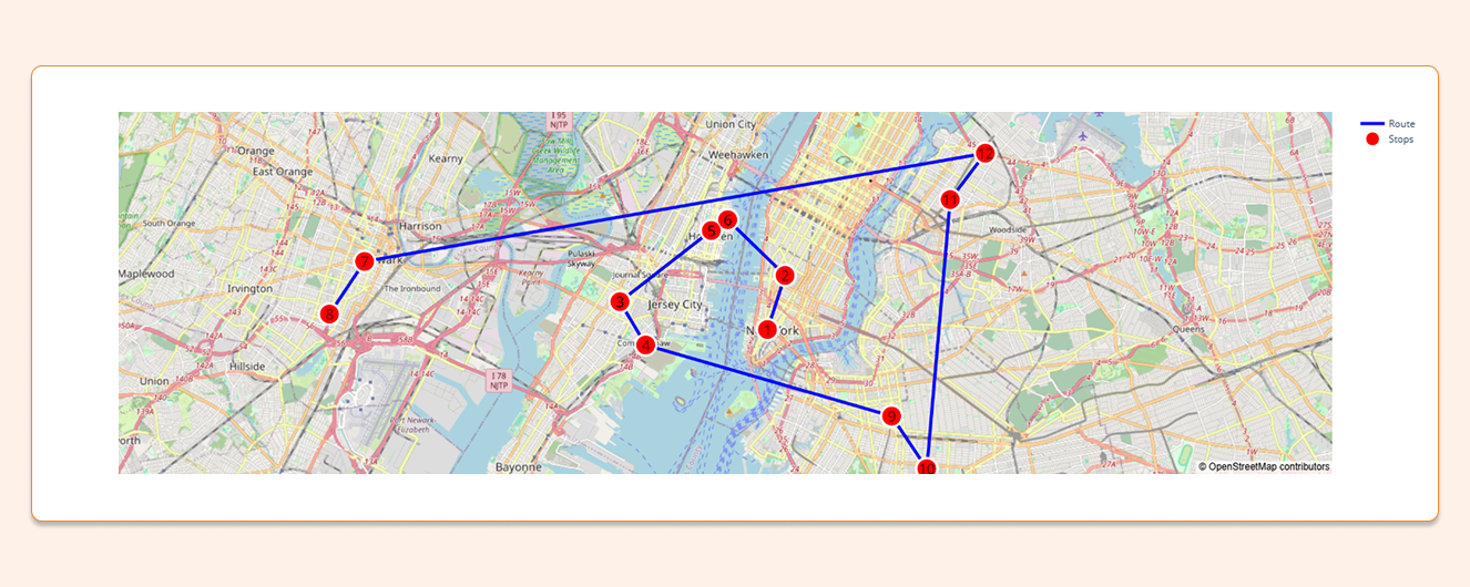
Visualization with Plotly
While I initially attempted to use Spark's native plotting capabilities, the complexity of map visualizations led me to use Plotly Express with toPandas() instead. Here's the code for displaying zones and points in a Databricks notebook:
%python
import json
import plotly.express as px

# Cities polygon data
pdf_cities = df_cities.toPandas()
# Delivery points data
pdf_pts = df_deliveries.toPandas()

# Build FeatureCollection for polygons
features = [
    {"type": "Feature",
     "geometry": json.loads(s),
     "properties": {"name": n}}
    for n, s in zip(pdf_cities["name"], pdf_cities["geo_json"])
]
fc = {"type": "FeatureCollection", "features": features}

# Center the map on the first polygon
ring0 = fc["features"][0]["geometry"]["coordinates"][0]
center = {"lon": sum(p[0] for p in ring0)/len(ring0),
          "lat": sum(p[1] for p in ring0)/len(ring0)}

# Create base map with polygons
fig = px.choropleth_mapbox(
    pdf_cities.assign(loc=pdf_cities["name"]),
    geojson=fc,
    locations="loc",
    featureidkey="properties.name",
    color="loc",
    mapbox_style="open-street-map",
    center=center,
    zoom=10,
    opacity=0.55
)

# Add delivery points as markers
fig.add_scattermapbox(
    lon=pdf_pts["lon"],
    lat=pdf_pts["lat"],
    mode="markers",
    text=pdf_pts["id"].astype(str),
    name="Deliveries",
    marker=dict(
        size=16,
        sizemode="diameter",
        color="red"
    )
)

# Render in Databricks
displayHTML(fig.to_html(include_plotlyjs="cdn", full_html=False))
Final Thoughts
Databricks Runtime 17.1's geospatial capabilities open up powerful possibilities for location-based data analysis. From simple spatial joins to complex routing algorithms, these new features make geographic data processing more accessible and efficient than ever before. Whether you're optimizing delivery routes, analyzing customer distribution, or performing spatial analytics, these tools provide the foundation for sophisticated geospatial applications.